Sunday, October 27, 2013

Fourier Pumpkins


In honor of Halloween, we thought a picture of a pumpkin would be fun. But how to make it "mathy?"

We started with the following picture of a pumpkin, found through a Google image search for "pumpkin clip art." We then turned it into a black & white image, where the edges are accentuated:


To make the right hand image, we followed instructions found at a great blog post called "Making Formulas… for Everything—From Pi to the Pink Panther to Sir Isaac Newton," one of the many great posts found at blog.wolfram.com.

Continuing to follow the steps provided by the blog author Michael Trott, we used the latter image to create a set of points in the \(x\)-\(y\) plane. The points are subdivided into a set of curves (in this case, 8) and then approximated with a Fourier series. While it only takes 2 sentences to describe what we did, it took many, many lines of code provided by Mr. Trott. (We highly recommend downloading the .cdf provided by the link and running it in Mathematica. If you want to upload your own image and make your own curves, it helps to know that not everything that you run in the .cdf is directly related to making curves. It can be boiled down to a lot fewer lines of code - but it's still a lot.)

All of the above should make some ask "What is a Fourier Series?" In short, a Fourier series is a sum of sines and cosines used to approximate another function. Since trigonometric functions are used, Fourier series are especially good at approximating periodic (that is, repeating) functions. The more sines and cosines used, the better the approximation (in general).

For example, consider the curve on the left, below.


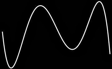
On the right, we approximate the curve with a set of Fourier series. We start with just \( 0.358+0.34\sin(1.28x)-1.03\cos(1.28x)\): that's the curve that is mostly flat. We then add more and more sine and cosine terms to better approximate the orginal curve. The 5th curve shown in the animation is \(0.358+\big(0.34\sin(1.28x)-1.03\cos(1.28x)\big) + \big(-5.34\sin(2.56x)+0.19\cos(2.56x)\big)\)
\(+\big(-1.88\sin(3.85x)+0.12\cos(3.85x)\big)+\big(-0.84\sin(5.13x) + 0.07\cos(5.13x)\big)\)
\(+\big(-0.44\sin(6.41x) + 0.05\cos(6.41x)\big)\)

To make the pumpkin, each of the 8 curves needed a different  number of sines and cosines to make it look good. The first part drawn, and by far the longest, needed the most: 180 sines and cosines!! We then plotted it for increasing values of \(t\), making it look it was being drawn.

The following animation shows how the approximation gets better and better by adding more and more terms to the series:


We thought another Halloweeny picture would be good. We did another Google image search, this time for "bat clip art", and came up with the picture below:


We followed the same procedure outlined by the Wolfram blog and made the following animations:


Finally, we thought the following image was pretty cool, suggested by another part of the Wolfram post. It shows, with increasing levels of opacity (i.e., the better the approximation the more opaque), various approximations of the bat by Fourier series.


So what good are Fourier series? Many of us view functions like \(1.03\cos(1.28x)\) as not-very-simple-or-intuitive. So why use them? There are 3 main reasons.

First, some problems involving functions are really hard to solve in general, but (amazingly) not so bad when the functions are trig functions. So approximating the real function with lots of trig functions (i.e., a Fourier series) makes finding an approximate solution easy.

Second, some data demonstrates oscillating, or periodic, behavior. (An easy example is sound waves.) One way of analyzing the data is to analyze the Fourier series that approximates it. We can also compress data this way - instead of storing all the information supplied by a sound wave, we can store only the Fourier coefficients, taking much less space.

Finally, Fourier himself was interested in approximating curves with sums of sine waves with the intent to draw cool pictures. He never went very far with it, though; on his death bed, he is reported to have said: "Si seulement j'avais animé une citrouille. Ensuite, ma vie aurait été complet," which translates roughly to  "If only I had animated a pumpkin. Then my life would have been complete."


Follow us on Twitter and we'll update you when a new post is up.


Sunday, October 20, 2013

Conformal Maps


Most people are familiar with basic functions like \(y=x^2\), and recognize its graph as the standard parabola. One thing we often don't consider is that this function is also a geometric transformation. That is, it takes the straight line segment [-1,1], for instance, and turns it a particular curve in the plane (that "starts" at (-1,1), passes through (0,0), and "ends" at (1,1)). All functions do this, in fact, some making more interesting--looking curves than others, especially if one considers parametric or polar functions.

Ultimately, though, we take a one-dimensional object (an interval of the \(x\)-axis) and transform it into another one dimensional object, a curve in the plane. One dimensional objects are so ... one dimensional. To make things more interesting, we should consider two dimensional regions of the \(x\)-\(y\) plane, and think of ways to transform them. 

There are infinitely many ways of doing this. One way is to pick two functions \(f\) and \(g\) and send the point \((x,y)\) to the point \((f(x),g(y))\). I thought of animating this for functions like \(f(x) = \sin x\) and \(g(x) = x^2\), but in general, this process makes a mess. (We'd love to see some people do this, though. If you do, share!)

A much, much better way of transforming the plane is through a linear transformation. It is pretty simple: pick 4 numbers \(a\), \(b\), \(c\) and \(d\) and map the point \((x,y)\) to the point \((ax+by,cx+dy)\).  This kind of transformation always sends straight lines to straight lines and circles go to ellipses. Relative distances are also preserved: if the point \(Q\) is 2/3 from \(P\) to \(R\), then \(Q\) gets mapped to a point 2/3 from where \(P\) and \(R\) get mapped to. 

These linear transformations are the underpinnings of computer graphics. For instance, letting \(a=\cos\theta\), \(b=-\sin\theta\), \(c=\sin\theta\) and \(d=\cos \theta\), we can rotate the point \((x,y)\) around the origin counterclockwise by the angle \(\theta\).  Below, we rotate the rectangle with corners (-1,0) and (1,1) around the orgin by 90\(^\circ\). On the left is the original rectangle, on the right is its transformation. Note how the shape and distances are all preserved.


Linear transformation on points \((x,y,z)\) in space allow one to rotate a 3D world, move through it, and show it all on a flat screen (Wolfenstein 3D, anyone?). The GPU's on computers are really, really, really good at performing these transformation fast.

Usually linear transformations do not preserve angles. That is, if two lines meet at a 15\(^\circ\) angle, the transformed lines probably do not meet at the same angle. This is ok for some applications, like projecting a 3D world onto your phone's screen. A map that does preserve angles is called a conformal map. 

To perform such a transformation, we need to view the \(x\)-\(y\) plane in a different way. We start with imaginary numbers. We first learned that \(\sqrt{4} = 2\) and \(\sqrt{-4}\) didn't exist. Later, some of us learned to give the expression \(\sqrt{-1}\) the name \(i\) and call it an imaginary number, as though it only existed in our minds. That allows us to get numbers like \(\sqrt{-4} = 2i\). With the basic principle that \(i^2=-1\), we can create complex numbers like \(2+3i\) and multiply them:
\[(2+3i)(1+2i) = -4+5i.\]

A complex function acts on these complex numbers. For instance, \(f(z) = z^2\) (we often use \(z\) for complex numbers) does the following:

\[ f(3) = 9,\quad f(3i) = -9\quad \text{and} \quad f(1+2i) = -3+4i, \quad \text{etc.}\]

We can visualize complex  numbers with the complex plane. Identify the complex number \(2+3i\) with the point (2,3) in the \(x\)-\(y\) plane. Each point in the plane represents a complex number. Tons of cool stuff comes out of this. 

A great result is that we can now transform this complex plane by applying a complex function to every point (i.e., every complex number) in the plane. 

We now reward to reader who has read this far with some more eye candy. In each of the following, we transform the same rectangle as before (now with vertices at \((-1,0)\sim -1\) and \((1,1) \sim 1+i\)) by a complex function. As you look at these, note how angles are preserved. In the rectangle, we have lots of right angles as the vertical and horizontal lines meet. In the transformed shapes, all the new curves intersect each other at right angles. (You should find that amazing. I do.)

Our introductory image was \(f(z) = e^z\):


We also have \(f(z) = 2 \sqrt{z + 1} +\frac{\ln(\sqrt{z + 1} - 1)}{\sqrt{z + 1} + 1}\)


\(f(z) = \sqrt{z}\): 


\(f(z) = \sin z\):


A really cool thing is that rotations are just multiplications by complex numbers. To rotate and scale, multiply by any complex number; to just rotate, multiply by a complex number of the form \(\cos \theta + i\sin \theta\).  A 90\(^\circ\) rotation is just a multiplication by \(i\), as seen before:

\(f(z) = iz\):


A basic shift up is done by adding \(i\) to every number/point:

\(f(z) = i+z\):


One final one for fun:

\(f(z) = (1+i+z)^2\):


What good is any of this? Two quick answers:

1. What good is this?!?! Are you kidding me? This is awesome. We just took a rectangle, deformed it in weird ways, but preserved angles. Who would have thought this was possible?!?

2. There are many problems in physics/engineering that depend on complex (no pun intended) geometry - for instance, fluid flow around corners or obstacles. The right conformal map can transform the complicated geometry into a simpler geometry, where the problem is "easy" to solve. This solution can be transformed back into a solution in the original geometry using the inverse conformal map. 

While we are pleased that #2 is possible, we here are more impressed by answer #1. 

A final note: this post was inspired by a reader comment. We probably misunderstood the comment, but we rotated a shape by moving points in a straight line and wondered if the reverse was possible - can we move a shape in a straight line by rotating its points? A comment suggested using an inversion (or see this), which got us thinking about conformal maps. So thanks for the comments - we like them and they give us ideas.

Oh - and someday, we'll post the code for our images. These .gif's were produced mostly on a Friday afternoon when we should have been grading papers or writing Chapter 13 of our Calc III book. Our code is generally ugly -  we write stuff in whatever way seems easiest at the time, and only figure out how to make it look nice and readable much later. So ... later we'll post some code because we do want to share.


Sunday, October 13, 2013

Rotations Through Translations


Looking closely, you'll notice that while this shape rotates, it is made up of individual points that do not rotate, but rather each moves along its own line. So the shape is made up of a bunch of points; the shape rotates, but each points translates.

This picture was inspired by this link, shared by my friend at  @mathawakenings. I'm not sure who made that image first. I was intrigued by it, and several days later, attempted to make it myself.

If you are not convinced that each point only moves along a line, consider the following image, where each point is colored:


That was my attempt to imitate the original image. I realized later that mine is different than that original post in several ways, including the cool motion-blur effect on the dots. Maybe I'll figure that out later.

If you are still unconvinced that each point only moves along a line, try this last image:


It is easy to just follow the red dot and see it travels along a line.

Making the image wasn't too hard to do, though I didn't have immediate success. Apart from a few abject failures, this was the first "successful" animation I made:


It looked cool, though not exactly what I wanted. I went ahead and made a color version of it too:


Again, one can follow a single color and see that each point moves along a line. For the skeptical:


This image gives the impression that we have one circle rolling around inside a second larger circle. Picking one point on the interior circle and following its path creates a curve called a hypocycloid  For instance, with an outer circle with radius 2 and an interior circle with radius 0.3, we get:


As a kid, I had a Spirograph with which I tried making similar curves. (I found it both really cool and really frustrating for my young/little mind/hands.)

Is there a hypocycloid where each point on the interior circle just travels in a straight line? Indeed, there is: let the interior circle have half the radius of the outside circle:


Each of the two rotating shapes shown here (the circle and the original shape) are examples of rose curves. They can be created with a certain (integer) number of petals with the polar equation r=sin(nt). If n is odd, the curve has n petals; if n is even, the curve has 2n petals. (This makes it hard to get a curve with six petals.)

Here is a sneaky way of seeing that each point in the 3-petal curve above actually moves in a straight line. The curve is defined by r=sin(3t); each point on the curve corresponds to a specific value of t. We can rotate any given shape by adding to the angle (if r=f(t), then r=f(t+a) rotates the shape clockwise a radians/degrees). 

To rotate the 3-petal curve, add a to the angle: r=sin(3t+a). This also accomplishes something else: if we think of a specific t value, adding a to the angle changes how far (r) the point is from the origin. In polar terms, we are still "looking" in the "t" direction, but just at a different  length than before. Moving in the same direction, but at different distances, means one is moving along a line.

So we can move a shape by translating its points. I made rose curves with various number of petals, but I think the 3-curve hits the sweet spot for beauty and simplicity. 

Here is the challenge: can one create a shape that translates by each of its points rotating in a circle? I played with the notion for a while, but my brain began to hurt. I'd like to see an example, or a clever proof showing it can't be done.


Friday, October 4, 2013

Reflective Property of the Parabola


All rays emanating from the focus of a parabola reflect off the parabola along parallel lines (each perpendicular to the parabola's directrix, not shown). 

Note how each ray "lines up" with the other rays after it has reflected off the parabola. The reason for this is related to the fact that rays emanating from one focus of an ellipse arrive at the other focus at the same time, illustrated in this post

A parabola is just a special ellipse. A parabola does not have just one focus; rather, it has two, but the other is located "at infinity." A future post will illustrate how an ellipse can be stretched to form a parabola. Therefore all rays emanating from "the" focus of a parabola travel toward the other focus (at infinity) and will arrive there at the same time, just as happens in the ellipse. 

Of course, this can sound like pure silliness - after all, what does it mean to "arrive at infinity at the same time"? One can rigorously defend this statement using limits, which might make for an interesting animated gif ...